Toolbox 1
Copy Exact Formula
Use the tool to copy the exact formula from a cell or range without altering any references. You can then paste the formula using CTRL+V.
Fix Formula References
Convert formula references to absolute so they remain unchanged when copied to other cells.
Unfix Formula References
Convert formula references to relative so they adjust automatically when copied to other cells.
Add IFERROR to Formula
Add IFERROR functions to the formulas in the selected cells for consistent error handling. Note: You can customize the error output via Settings.
Remove IFERROR from Formula
Remove IFERROR functions from the formulas in the selected cells.
Multiply by
Multiply selected formulas or values by a value.
Divide by
Divide selected formulas or values by a value.
Add Percentage of Total
Insert percentage formulas by dividing a selected range of cells by a specified row.
Tip: Use this tool not only for % of total calculations but also to effortlessly add 'percentage of revenue' KPI formulas.
Add Difference
Quickly insert formulas to subtract one range of cells from another.
Add CAGR
Add a compound annual growth rate (CAGR) formula.
Swap Formulas Between Two Ranges
Swap contents between two cells or ranges without the need for temporary storage.
Add Text to Formula or Value
Insert text at the beginning or end of existing cell contents (formulas or values).
Tip: Perfect for adding an apostrophe (‘) to enforce text formatting or for inserting a cell reference (e.g. including an FX rate) across multiple cells at once.
Add Period Name Labels
Generate monthly period name labels like 'Jan-24', 'Jan24', or '31/01/2024'.
Each selected cell will be filled with the next consecutive period label. You can choose between text or date formatting. Tip: For consultants, we usually recommend text formatting to ensure consistent date display across different regional settings and user preferences.
Add HyperLink to Cell Reference
Add a hyperlink to a cell that directs to the first cell reference in its formula.
Many Excel users have the option to jump to the first cell reference by double-clicking a cell disabled. To bypass this, you can use this utility to create a hyperlink that takes you directly to the location you would normally reach by double-clicking the cell.
Bring Formula Forward
Replace the first cell reference in a formula with its underlying formula or value.
You can use this tool to simplify formulas in certain circumstances.
Send Formula Backward
Send a formula or value to a formula’s first referenced cell.
This tool lets you apply changes across multiple cells without the hassle of manually navigating to each one. For example, you can update titles on multiple sheets or modify cells with specific filter conditions in one go. Tip: Pair this with Sheet Links to easily manage and export cell locations.
Fill Empty Cells with Zeros
Fill empty or blank cells in the selection with zeros.
AutoFill Cells
Fill empty cells with contents from preceding non-empty cells from different directions.
Toolbox 2
Highlight Duplicates
Identify duplicate values in selected cells without relying on conditional formatting. Tip: Conditional formatting can be resource-intensive and may slow down your workbook, so it's best to use it sparingly.
Highlight Differences
Find differences between ranges: items unique to each range are highlighted.
Insert Rows
Insert multiple rows based on the following scenarios:
Single range selection: Count the number of rows in the selection and insert that many rows after a specified cell.
Multiple range selection: Insert a specified number of rows after each selection.
Insert Columns
Insert multiple columns based on the following scenarios:
Single range selection: Count the number of columns in the selection and insert that many columns after a specified cell.
Multiple range selection: Insert a specified number of columns after each selection.
Apply Row Groups/Outline Based on Indentation
Automatically add row groups/outline based on existing cell indentations.
Apply Indentation Based on Row Groups/Outline
Automatically add cell indentations based on existing row groups/outline.
Apply Row Groups/Outline & Indent from SUM/SUBTOTAL
Automatically add row groups/outlines and cell indents based on the hierarchy implied by existing SUM or SUBTOTAL functions.
For fine-tuning, use 'Formats' > 'Add Hierarchy Level' or 'Remove Hierarchy Level'.
Add 'Subtotal Lines' to Row Groups/Outline
Add a collapsible visual separator between the subtotal and detail rows across the selection.
Note: The bottom border is applied to the row right before a change in the row group level, but only for collapsible groups (outline levels > 1).
Remove 'Subtotal Lines' from Row Groups/Outline
Remove 'Subtotal Line' formats from collapsible rows.
Note: All borders are removed from collapsible row groups (outline levels > 1).
Text Utilities
Center Across Selection
Use this to create a label that spans multiple columns without merging cells, as merging cells should be avoided when possible.
Trim Text / Remove Leading and Trailing Spaces
Remove unwanted spaces from the beginning and end of the text in each selected cell.
Convert Text to Upper Case
Convert text in each selected cell to upper case.
Convert Text to Lower Case
Convert text in each selected cell to lower case.
Convert Text to Sentence Case
Convert the first letter of the first word in each selected cell to upper case.
Convert Text to Title Case
Convert the first letter of every word in each selected cell to upper case.
Formats
The Formats menu offers quick and intuitive access to commonly used formatting options, allowing you to apply them efficiently without extra steps or overriding Excel’s native keyboard shortcuts.
For example, you can apply the customizable 'Total Row' format to your selection using:
- Accelerate Ribbon: Alt > G > 3 > T
- Quick Access Toolbar: Alt > 1 > T
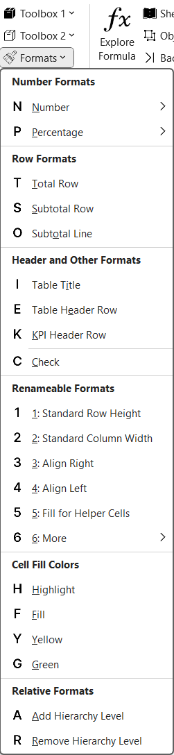
These fully customizable formatting options are inspired by the most commonly used styles in transaction advisory. Plus, you have ten additional formatting shortcuts, labeled as ‘Renameable Formats,’ which you can rename as you like.
In the toolbar’s Settings, you can completely customize all formats (except for ‘Check’) using the following options:
Number Format
Alignment: Horizontal, Vertical, Indentation
Font: Name, Size, Italic, Bold, Underline, Color, Effects
Borders (Top, Bottom, Left, Right): Color, Style
Fill: Color, Pattern Color, Style
Row Group/Outline Level
Column Group/Outline Level
Row Height/Column Width
Increase/Decrease Row/Column Group Level and/or Indentation