How to Master Power Pivot in Excel
What is Power Pivot?
Power Pivot is an Excel add-in and data analytics tool that has been pre-installed in Microsoft Excel since 2013. It allows you to analyze your data and gain meaningful insights. If you're familiar with Pivot Tables, think of Power Pivot as a more advanced version. Unlike Pivot Tables, which are limited to a single data table, Power Pivot allows you to analyze large datasets across multiple tables, making it increasingly valuable in the world of big data.
Table of Contents
Work Faster with Accelerate Excel
Simplify your Excel work with the Accelerate ribbon comprising tools for M&A Transaction/Deal Advisory, FDD and other Excel power users.
How to Get the Excel Power Pivot Add-In?
To access Power Pivot features, open an Excel workbook and go to File > Options.
In the newly opened window, select Add-Ins from the left panel.
In the Manage drop-down menu, select COM Add-Ins and click GO.
Check the box for Microsoft Power Pivot for Excel and click OK.
This will add the Power Pivot tab to your Excel ribbon.

Open COM Add-ins: File > Options > Add-ins > COM Add-ins
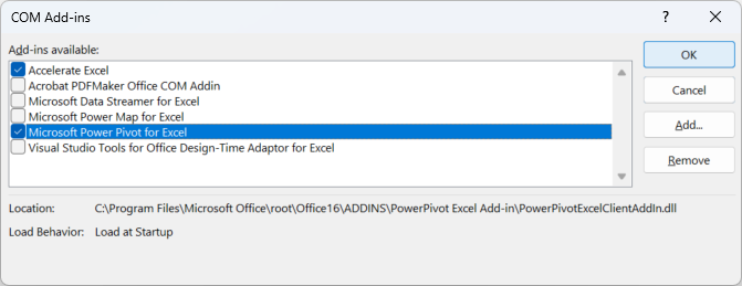
Enable Microsoft Power Pivot for Excel
Ready to Start Working with Excel Power Pivot?
The first step is to create a Data Model, which is a collection of tables or datasets. We'll use financial information to build our data model and establish relationships between the tables. You can use any type of data; we're just using financial data as an example. To create relationships later, ensure that the tables share at least one common field.
Step 1: Start by Opening the Power Pivot Window
Let’s get started! Open Power Pivot and click on Manage to access the Power Pivot window. Next, we need to bring in some data. Power Pivot allows you to import data from various sources. Whatever data you have, there's a good chance you can import it into Power Pivot using one of the available options:
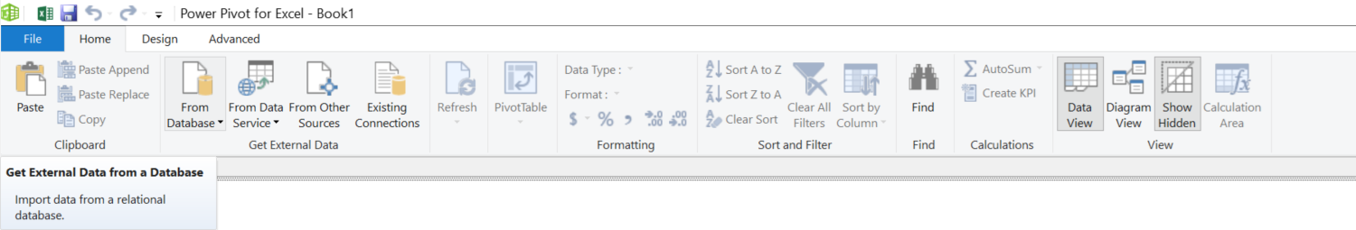
Open the Power Pivot main Window: Power Pivot > Manage > Home
Step 2: Import Data from Multiple sources:
From Databases (SQL Server, Microsoft Access or Analysis Services or PowerPivot)
From an OData data feed
From Other Sources (Oracle, Teradata, Sybase and more)
From Data Feeds
From Excel files
One of the key benefits of Power Pivot is its ability to simplify data management. Previously, combining data from multiple worksheets and sources often required manual effort, such as copying and pasting information or writing VBA code.
Step 3: Adding Data to the Data Model
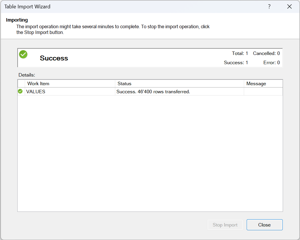
In our example, we'll use data from an Excel file. Here's how to import it:
Go to Get External Data > From Other Sources > Text Files > Excel File and click Next.
On the next screen, set a friendly connection name. We'll use "VALUES".
Select your Excel file by clicking Browse and navigating to the file. Start by selecting the VALUES.xlsx file and click Open.
Since our source file has column headers in the first row, check the option Use first row as column headers and click Next.
The next window will show the source table, in this case, VALUES. You can also use Preview & Filter to check your imported data.
If the data looks good, click Finish.
Finally, you can see how many rows were transferred. In our example, we successfully transferred 46,400 rows of data.
We’ve successfully imported the first source, which includes the account values and associated periods. However, the true strength of Power Pivot and the Power Pivot Data Model is its ability to connect multiple data sources. So, let’s bring in the remaining data.
Repeat the import process for the other two source files: MAPPING_ACCOUNTS.xlsx and MAPPING_PERIODS.xlsx. This will allow us to combine and analyze all relevant data within the Power Pivot model.

Open the Table Import Wizard: Get External Data > From Other Sources > Text Files > Excel File
Import the datasets through the Table Import Wizard
Step 4: Establish Relationships in the Data Model
After importing the data, you can not only view information from multiple sources simultaneously but also define relationships between them. For example, you’ll notice that the VALUES sheet contains a column called ID_ACCOUNT, which matches a column in the MAPPING_ACCOUNTS sheet. Similarly, there’s an ID_PERIOD column in both VALUES and MAPPING_PERIODS. Excel doesn’t automatically recognize these relationships, so we need to define them ourselves.
To set up these relationships:
Go to the Home tab and click on Diagram View on the right-hand side. This view displays all the imported data and fields within each table.
Click on the column containing the related ID (e.g., ID_ACCOUNT) and drag it to the corresponding ID column in the other table. A line will appear to show the connection.
Release the mouse button, and you’ll see a relationship is created when you hover over the line.
Repeat this process to connect the ID_PERIOD from the VALUES table to the MAPPING_PERIODS table.
Once done, you’ll have established two relationships. If you need to delete a relationship, right-click on the line and select Delete.

Open the Diagram View: Power Pivot > Manage > Home > Diagram View
Data Modeling in Power Pivot: DAX Formulas & Measures and Sorting
DAX Formulas & Measures
Setting up the data model in Power Pivot is relatively simple and fast to execute. In our example, we've used source files containing all the relevant information we need. Another key advantage of Power Pivot is to manipulate data by adding new columns, known as calculated columns, using DAX (Data Analysis Expressions) formulas.
For instance, if you need to create a new measure that returns values in millions, you can easily do this in Power Pivot. Currently, the sum of values might return results in thousands, but you can create a new measure to convert these results into millions. Here’s how you can add a new measure:
For more complex calculations, DAX offers powerful functions. For example, if you have sales data and you want to create a measure for total sales of a specific product type, such as "new," you can use the following DAX formula:
These calculations in Power Pivot are similar to Excel formulas but work directly within the data model, allowing you to create new fields and measures with just a few clicks. A common example is calculating Key Performance Indicators (KPIs) to track and measure performance against specific goals.
By leveraging DAX, you can transform your data model into a powerful analytical tool, enabling data analysis and reporting. Whether creating simple calculated columns or complex measures, DAX provides the flexibility and functionality to maximize your data's potential.
For a comprehensive list of DAX functions, visit the DAX Function Reference.
Sorting
In Power Pivot, sorting one column by another is a powerful feature that ensures your data is organized exactly how you need it. This is especially useful when creating PivotTables from your data model, as pre-sorted data eliminates the need for manual sorting in the PivotTable.
For example, we have account names at different levels (L1, L2, L3...) and want them in the correct order for a P&L statement. By including a sort column, we can easily sort each account name by this accompanying column. Similarly, for our MAPPING_PERIOD, sorting these ensures our P&L is in chronological order.
Another use case is sorting product categories by their sales rank, ensuring the highest-selling products always appear first. Sorting columns by other columns in Power Pivot enhances data presentation and accuracy, making your analysis more effective and meaningful.
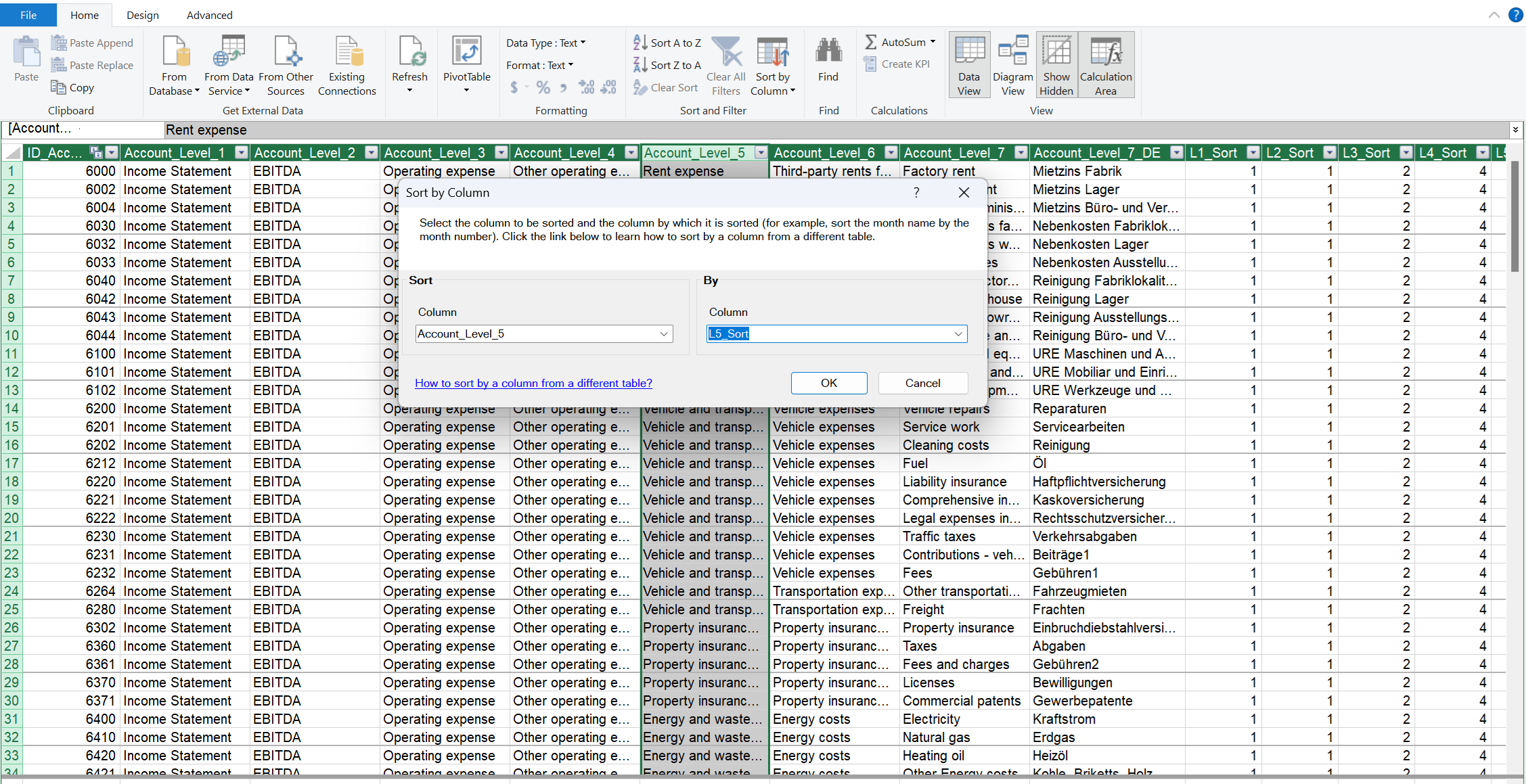
Sort by Column: Power Pivot > Manage > Home > Sort by Column
Create Pivot Tables Using Data Models
Once you have imported all datasets and added relevant DAX formulas to your Power Pivot, you can create PivotTables using your Data Model. This allows you to visualize your data and include other visual elements such as PivotCharts.
To add a PivotTable:
Click on Insert > PivotTable > From Data Model.
The Create PivotTable dialog box will appear. Select New Worksheet and click OK.
Now, let’s create a PivotTable using the data model to display the company P&L. Drag the relevant items into the appropriate areas (Rows, Columns, Values).

Drag and Drop the Pivot Fields in the correct areas: Insert > Pivottable > From Data Model
You can also add slicers to dynamically filter data based on selected criteria. A slicer acts like a visual filter for your data columns but is much quicker and more interactive. For example, add a slicer for the entity name to switch between different companies' P&Ls. To add a slicer, right-click on the field you want to filter by and select “Add as Slicer.”
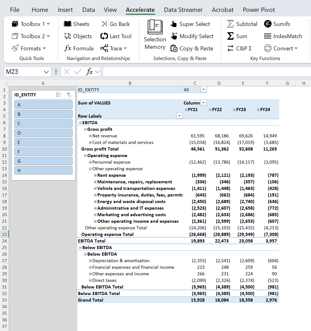
Sample Pivot Tables using the tutorial dataset
Understanding OLAP Conversion: Improving Pivot Table Flexibility
While Power Pivot offers powerful data modelling and analysis capabilities, a common limitation is the formatting flexibility of PivotTables. To overcome this, you can convert a PivotTable into CUBE functions using OLAP (Online Analytical Processing). This conversion transforms the data model into an OLAP cube, which maintains high performance while providing greater formatting flexibility for your reports. By leveraging OLAP cubes, you gain the ability to format your data just like regular Excel cells, addressing the flexibility issues of traditional PivotTables. For further insights into OLAP and CUBE functions and a tutorial on how to automate the formatting process using the Accelerate Excel add-in, you can explore more detailed information in our next article.

OLAP Converstion: PivotTable Analyse > OLAP Tools > Convert to Formula
Conclusion
In this article, we explored Power Pivot and its capabilities through a practical example. You learned how to import data into your data model, establish relationships, create measures using DAX, and sort and use data in PivotTables.
However, you might be curious about how Power Pivot stacks up against other data analysis tools like Power Query and Power BI. Here’s a brief overview to help clarify their roles and how they complement each other:
Power Query: This is powerful when it comes to data collection and preparation. It offers a user-friendly interface for importing, transforming, and cleaning data before it enters your data model. While Power Pivot handles data modelling and analysis, Power Query specializes in shaping and loading data efficiently. These tools often work together, with Power Query managing data preparation and Power Pivot focusing on the data model and analytical tasks.
Power BI: Power BI combines the functionalities of both Power Query and Power Pivot and adds advanced capabilities for creating interactive reports and dashboards. It allows you to publish reports to the cloud for real-time data access and sharing, making it a comprehensive solution for business intelligence and data visualization.
Choosing Between Power Pivot and Power BI: Power BI encompasses the same data modelling and DAX formula capabilities as Power Pivot but also includes enhanced reporting features and cloud integration. If your primary need is data modelling and analysis within Excel, Power Pivot may suffice. However, for a more extensive solution with advanced reporting and cloud functionalities, Power BI is the superior choice.
In summary, Power Pivot is a robust tool for data modelling in Excel, Power Query is perfect for data preparation, and Power BI offers a full suite for data analysis, reporting, and cloud integration. Each tool has its unique strengths, and using them together can greatly boost your data analytics capabilities.
Have questions or thoughts? Share them in the comments section below, and we will be happy to assist you!